The Mitosius

Creating the Mitosius is the last preparation step before the reconstruction. This section covers how to prepare the mitosius.

You have already run the coil sensitivity estimation or had an estimate of coil sensitivity by your own procedure (see the Coil Sensitivity Map Estimation). You need to have access to the raw data of the acquisition (of course :)).

This script is designed to process Siemens raw MRI data/ISMRMRD using various monalisa functions to load raw data, initialize parameters, compute trajectory points and volume elements, normalize the data, and generate the output “mitosius”. The resulting mitosius contains raw data, the computed trajectory and the volume elements for each bin.

Important

Keep in mind that the trajectory must be supported by the toolbox; alternatively, you can define and implement a custom trajectory following our suggestion at the end of the section (see the section Custom Trajectories).

Prerequisites

Ensure you have the following files and paths correctly set up:

• Siemens raw data file. (Or ISMRMRD file)

• Precomputed coil sensitivity matrix (C.mat).

• Precomputed binning mask (Mask.mat)

Additionally, the required functions (e.g., bmTwix_info, bmTwix, bmTraj, etc.) should be available in your MATLAB environment, as these functions are internal functions in the monalisa toolkit.

Tip

If you use a 3D radial trajectory, you can use bmTwix_info function to help you inspect acquisition parameters by bmTwix_info(‘/path/to/raw_data.dat’). bmTwix_info is only a help function which is not part of the recon procedure. Sometimes, bmTwix_info may fail to read the raw data file. But there is no need to worry-you can still find your way to identify acquisition parameters.

Usage instructions

Define the Paths

%% Paths - Replace for your own case
f = '/your/path/to/raw_data/rawdata.dat';
CMatPath = '/your/path/to/C/C.mat';
MaskPath = '/your/path/to/Mask/Mask.mat';
mitosiusPath = '/your/path/to/save/mitosius/';

Load the Raw Data

autoFlag = false;      % Set whether the validation UI is shown
% Create the appropriate reader based on the file extension
reader = createRawDataReader(f, autoFlag);

In our examples, we often use 3D radial trajectory. In that case, the raw data reader will check the first segment of each shot to estimate after how many nLines, steady state is reached. For your own trajectory, you can find your own way.

(The image title is yet to change)

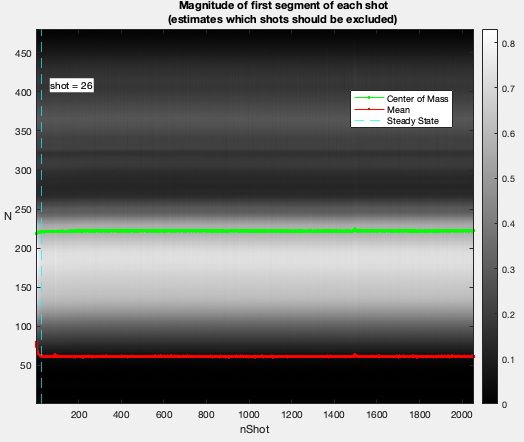
The acquisition parameters will be extracted automatically, if possible.

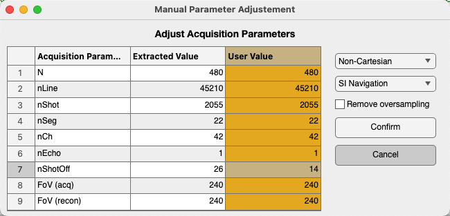
You can also modify the parameters manually in the “User Value” column (in yellow), for example: adjusting nShotOff according to your needs. If you want to include all the lines for reconstruction, set nShotOff = 0. Then click the “Confirm” button.

Add MRI Acquisition Parameters

Save the acquisition parameters into p and add other parameters you may need.

p = reader.acquisitionParams;
p.selfNav_flag = true;
p.traj_type = 'full_radial3_phylotaxis';

% Initialize and fill in the parameters:
% p.raw_N_u: acquisition matrix size (identified from your acquisition protocol)
p.raw_N_u         = [480, 480, 480]; % optional, just for records
p.raw_dK_u        = [1, 1, 1]./480; % optional, just for records

Read the raw data and compute trajectory points, volume elements

% Read raw data
% get raw data without nshotoff and SI
flagSS = true
flagExcludeSI = true
% flagSS: if true, filter out the non steady state shots
% flagExcludeSI: if true, filter out the SI projections
y_tot = reader.readRawData(flagSS, flagExcludeSI);

% compute trajectory points
% get 'full_radial3_phylotaxis' trajectory without nshotoff and SI
t_tot = bmTraj(p);
% alternatively you can compute your own trajectory
% more details in "Using a Custom Acquisition Trajectory" %TODO: correct ref

% compute volume elements (3D full radial trajectory in this case)
ve_tot  = bmVolumeElement(t_tot, 'voronoi_full_radial3');

Load the Coil Sensitivity Matrix

Resize the coil sensitivity matrix to match the reconstruction matrix size.

Tip

Here we want to clarify the distinction of the concepts between “Reconstruction matrix size” and “Acquisition matrix size”

• Acquisition matrix size: This refers to the matrix size specified by the acquisition protocol. It was already set at the acquisition step by the experimenters.

• Reconstruction matrix size Matrix_size: This is set by the user based on the desired resolution of reconstructed images, i.e. the size of the reconstructed image.

• N_u: The size of reconstruction grid in Fourier space. For example, we can set N_u = Matrix_size.

  • \(N_u = [N_x, N_y, N_z]\)

• n_u: The size of reconstruction in image space. It is possible to set n_u ≤ N_u. However, we recommend setting n_u = N_u for achieving the optimal image quality.

  • \(n_u = [n_x, n_y, n_z]\)

• dK_u: The step size of the grid in Fourier space, calculated as dK_u = 1/Fov.

  • \(dK_u = [dK_x, dK_y, dK_z]\)

load(CMatPath);
% n_u: reconstruction matrix size
C = bmImResize(C, [48, 48, 48], [N_u, N_u, N_u]);

Normalize the data

Normalize the raw data by the average value of a region of interest (ROI). The goal is to adjust the intensity values of the image so that they are centered around a mean of 1 in the ROI.

Important

Keep in mind that whether or not normalization is applied, the regularization weight in the final reconstruction step should be adjusted accordingly. Our normalization helps standardize the regularization weight.

x_tot = bmMathilda(y_tot, t_tot, ve_tot, C, N_u, n_u, dK_u);
bmImage(x_tot);
temp_im = getimage(gca);
bmImage(temp_im);
temp_roi = roipoly;

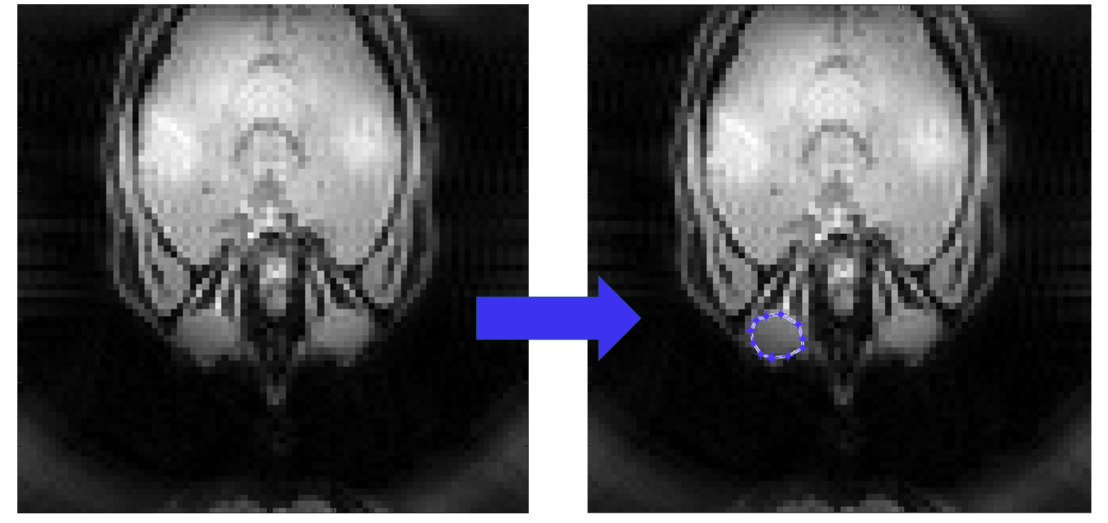
Here an estimation of the reconstructed image will be shown and you can select the ROI based on it.

We selected the left eye globe as the ROI in our example below, you can also select yours with a larger area in the brain.

• Left Click: Adds a vertex at the clicked position.

• Right Click/Double Click: Completes the polygon and closes it automatically.

normalize_val = mean(temp_im(temp_roi(:)));
% normalize it only once
y_tot = y_tot / normalize_val;

Cleaning of the mask

For some trajectories, such as the 3D radial trajectory, it is necessary to clean the SI projection and remove the first unsteady shots from the acquired readouts. Therefore, we also need to clean the binning mask accordingly to ensure that the size of Mask matches the size of y_tot.

load(MaskPath);
Mask = reshape(Mask, [20, 22, 2055]);
% before cleaning, the size of Mask: [nBin, nSeg, nShot]
Mask(:, 1, :) = [];
Mask(:, :, 1:p.nShot_off) = [];
% after cleaning, the size of Mask: [nBin, nSeg-1, nShot-p.nShot_off]
Mask = bmPointReshape(Mask);
% after the reshape, the size of Mask: [nBin, nLines]
% where nLines=(nSeg-1)*(nShot-p.nShot_off)

Compute Final Data Structures for Reconstruction

Run the bmMitosis function and compute the final volume elements.

[y, t] = bmMitosis(y_tot, t_tot, Mask);
y = bmPermuteToCol(y);
ve = bmVolumeElement(t, 'voronoi_full_radial3');

Save the Results

Save the computed data structures to disk. These will be used for the final reconstruction.

bmMitosius_create(mitosiusPath, y, t, ve);

Notes

• Ensure all paths are correctly set according to your system.

• If you encounter issues with function calls (e.g., bmTwix, bmTraj), verify that the necessary scripts or external toolboxes are added to the MATLAB path.

• The raw data normalization step ensures that the average value in the selected ROI ranges around the mean of 1 in the reconstructed images. This allows the standardization of the regularization weights.

↑