Sketching a Classical Thermodynamic Theory of Information for MRI Reconstructions
Introduction
The present section is a non-formal essay to sketch some basic features of what could be a thermodynamical theory of MRI reconstruction, or more generally, a thermodynamical theory of information for iterative algorithms.
Our idea is to convince the reader that a general picture may be sketched in the future, which includes MRI reconstructions, an entropy notion, computers, electrical power, reconstruction time, information gain, and artificial intelligence. Placing Monalisa in that picture allows in particular to understand the intuition that motivated the design of our toolbox: to efficiently consume a maximum amount of energy with a high-performance computer (HPC).
What we do in fact in this text is an analogy between a heat engine and a computer. In particular, we find a way to describe a computer performing an MRI reconstruction in the same way that a heat engine is compressing an ideal gas in a cylinder. We try to describe an iterative reconstruction as a machine that compresses the space of the dynamical variables of the reconstruction, and thus lowering the entropy of the computer memory in the same way that a each engine can lower the entropy of an ideal gas.
As the reader will notice, this discussion can be applied to any iterative algorithm that solves an inverse problem. The MRI reconstruction process is used here as a representant example for any iterative inverse-problem solving process. Given the generality of the statements exposed in this discussion, we can consider it as an attempt to formulate a classical (non-quantum) physical theory of information. In the discussion section, we will make some connection with the of Landauer’s principle, which makes the bridge between physics and information theory by providing an equivalence between energy and information.
Iterative Reconstructions
Before anything, we would like to indicate that the MRI reconstructions under consideration here are iterative reconstructions. These reconstructions appeared historically as iterative algorithms to find a minimizer of the non-constrained optimization problem
where \(FC\) is the linear model of the reconstruction, \(X\) is the set of MRI images, \(x\) is the candidate MRI image, \(Y\) is the set of MRI data, \(y\) is the measured MRI data, \(\lambda\) is the regularization parameter, and \(R\) is a regularization function with some nice properties (typically is \(R\) chosen to be proper closed convex). The objective function of the above optimization problem is made of
a data-fidelity term, which is small when the modeled data \(FCx\) is close to the measured data \(y\),
a regularization term, which is small when the image \(x\) is close to satisfying some prior-knowledge.
In this formalism, the choice of a regularization function implements a choice of prior-knowledge.
This argmin-problem is the conventional modern formulation of the general MRI reconstruction problem as an optimization problem. For many choices of regularization function, the reconstruction problem has some minimizers and there exists some iterative algorithm that converge to one of the minimizers, which depends usually on the initial image guess. The iterative algorithms that solve the above argmin-problem are the conventional iterative reconstruction methods. In addition to these conventional methods, some heurisitcs methods are inspired from the conventional ones but perform some heuristic update of some dynamical variables at each iteration. These methods converge in some cases but they do not minimize a given objective function and their convergence is not necessarily guaranteed by any mathematical formalism. Some examples of such heuristic reconstruction are iterative methods where some updates of the image or other dynamic variables are done by a statistical model. It is an example of use of artificial intelligence for MRI reconstruction.
Heuristic or not, we consider in the following iterative reconstructions that converges for some given dataset. From the view point of discrete dynamical system theory, we can summarize an iterative reconstruction as follows. An iterative reconstruction is given by a map \(\Phi\) from \(X \times Z\) to \(X \times Z\), which is parametrized by a list of scalar parameters param and the measured data \(y\), that we also consider as a parameter. Here is \(X\) the vector space of all MRI images of a given size, and \(Z\) is the cartesian product of all spaces that contain all other dynamical variables that we will write as a single list \(z\). We consider that a scalar parameter is a constant, known, controlled number and \(param\) is the list of those. It includes for example the regularization parameter \(\lambda\).
It holds then
Note that we write parameters after the “;” and the dynamical variables before.
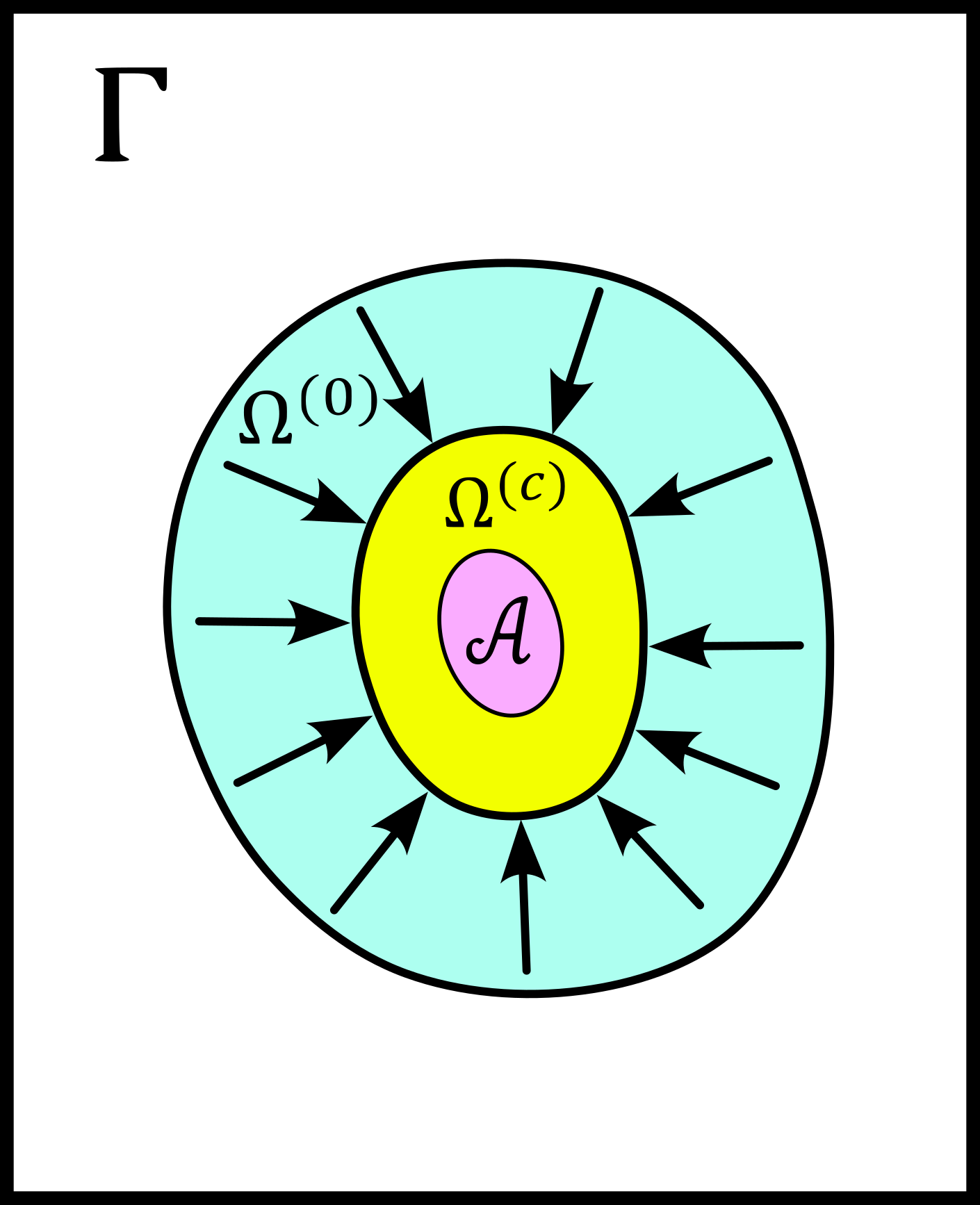
We expect from that dynamical system that for any initial value \((x^{(0)}, z^{(0)})\) the sequence converges to a pair \((x^{(inf)}, z^{(inf)})\), which may depend on the initial value. The set of all limits is the attractor of the dynamical system, that we will write \(\mathcal{A}\). The stability of each element a of the attractor may then be analyzed by the tool of dynamic system theory. But from the point of view of application, it makes sense to assume the attractor to not be chaotic. Note that in practice, the attractor is larger than a single point and the bassin of attraction \(\mathcal{B}(a)\) of an element a of the attractor (the set of initial values that lead to a sequence converging to a) is also lager than a single point.
For a given objective function to minimize, the art of building an algorithm that finds a minimizer consists of building a map \(\Phi\) for which the projection of its attractor on the space \(X\) co-inside with the set of minimizer of the objective function (or a subset of it). But as we said, some heuristic iterative reconstruction algorithms are not finding some minimizer of any objective function. We will therefore consider the projection of \(\mathcal{A}\) on \(X\) as the set of possible reconstructed images.
We further would like to point out that a non-iterative (single step) reconstruction can be seen as an iterative reconstruction. For that, we only have to realize that a non-iterative reconstruction is given by a map \(\phi\) that does not depends on \((x, z)\):
In that sense, all reconstruction are iterative, and those we called “non-iterative” converge in a single step since
Iterative reconstruction guided by (based on, using, enhanced by…) an artificial intelligence of any kind can be seen as a dynamic system where the implementation of \(\Phi\) contains some statistical model. For example, if \(\mathcal{N}\) is a neuronal network trained to predict some of the dynamical variables from the measured data set and from a database of good quality images, it can be used to update that dynamical variable as each iteration. We can then see \(\mathcal{N}\) as a parameter of the map \(\Phi\):
In the following, we will not make a distinction between the image \(x\) and the list of other dynamic variables \(z\). We will write the current state of all dynamic variables as
The initial value \((x^{(0)}, z^{(0)})\) will thus be written \(\omega^{(0)}\) and the current list of all dynamic variables at step \(c\) will be written \(\omega^{(c)}\). Also, we will write the list of all parameters as a single list \(\theta\) such as
or
We can thus summarize an iterative reconstruction by the formula
In summary, an iterative reconstruction is a discrete dynamical system given by a map \(\Phi\) with a attractor \(\mathcal{A}\), where each element \(a \in \mathcal{A}\) has its own bassin of attraction \(\mathcal{B}(a)\).
The Phase Space
We define here our phase space of MRI reconstruction. For that, we will get some inspiration from the physics. The spirit of phase space in physics is the following. The phase space is a set so that each of its element corresponds to exactly one of the state that the physical system under consideration can occupy, and each of these element carries the complete information about the system occupying that state. In classical Hamiltonian mechanic for example, if one knows the position in phase space of a physical system at some time, then everything about the system is known at that time. In particular, it is then possible to predict all future states of the system and find all its past states. In our case of MRI reconstruction, the map \(\Phi\) that dictates the dynamic may not be invertible. We therefore cannot expect to recover the past history of a position in phase space, but at least its future states. It makes therefore sense to define our phase space as
The state of our system at a given time (a given iteration) is then given by a pair \((x, z)\) and its knowledge is sufficient to predict all future states by iterating \(\Phi\) on that pair. Note that the attractor \(\mathcal{A}\) is a proper subset of the phase-space \(\Gamma\). As said earlier, instead of writing \((x, z)\) we will just write \(\omega\). The phase space is therefore the set of possible \(\omega\) and the map \(\Phi\) is from \(\Gamma\) to \(\Gamma\).
We can reasonably assume that for any application, \(\omega\) can be considered to be a large array of \(n\) complex or real numbers. Since the theory of MRI reconstructions is naturally formulated with complex numbers, we will consider that
for a positive and even integer \(n\).
An iterative reconstruction process can then be described in two steps:
to choose an initial guess \(\omega^{(0)}\) in a set \(\Omega^{(0)} \subset \Gamma\).
to iterate \(\Phi\) on \(\omega^{(0)}\) until the obtained value \(\omega^{(c)} = \Phi^{(c)}(\omega^{(0)}; \ \theta)\) is sufficiently close to the attractor \(\mathcal{A}\).
Here is \(\Omega^{(0)}\) the set in which we allow to choose the initial values.
The description of the second step is however not appropriate to the thermodynamical description we are going to present. In order to prepare the rest of the discussion, we need to reformulate those two steps in term of sets and distributions. For a given subset \(\Omega \subset \Gamma\) we define
As already said, our phase space \(\Gamma\) can be considered as isomorphic to \(\mathbb{R}^n\) for some positive integer \(n\). We can thus consider that \(\Gamma\) can be equipped with the \(\sigma\)-algebra of Lebesgue measurable sets, that we will write \(\mathcal{L}\), so that \((\Gamma, \mathcal{L})\) is a measurable space. We further provide this measurable space with the Lebesgue measure that we will write \(\lambda\) to obtain a measure space \(\left( \Gamma, \mathcal{L}, \lambda \right)\).
We will write \(\Omega^{(c)}\) the subset of \(\Gamma\) defined by
It is the set that contains \(\omega^{(c)}\), whatever the initial value of the reconstruction process, as long as it is in \(\Omega^{(0)}\).
Note that given the subset \(\Omega^{(0)} \subset \Gamma\), the set of parts
is a \(\sigma\)-algerba on \(\Omega^{(0)}\). More generally, for a subset \(S \subset \Gamma\) we will define the \(\sigma\)-algerba \(\mathcal{L}\left(S\right)\) as
Let be \(\tilde{\mu}^{(0)}\) a probability measure on \(\Omega^{(0)}\) with probability distribution function (PDF) given by \(p_{\tilde{\mu}^{(0)}}\) so that the probability that the random variable associated to \(\tilde{\mu}^{(0)}\) appears in a set \(\Omega \subset \Omega^{(0)}\) is given by
It means that \(p_{\tilde{\mu}^{(0)}}\) is the Radon-Nikodym derivative of \(\tilde{\mu}^{(0)}\) with respect to \(\lambda\). It holds in particular
so that the triple \(\left( \Omega^{(0)}, \mathcal{L}\left(\Omega^{(0)}\right), \tilde{\mu}^{(0)} \right)\) is a probability space (i.e. a measure space where the measure of the entire set is 1). The following figure summarizes the situation.
We now reformulate the two steps of an MRI reconstruction process as follows:
Instead of choosing an initial guess, we chose a probability measure \(\tilde{\mu}^{(0)}\) as above so that the initial value \(\omega^{(0)}\) is a random variable with PDF equal to \(p_{\tilde{\mu}^{(0)}}\).
We describe then the iteration process as a contraction of \(\Omega^{(0)}\) by iterating on it the map \(\Phi\) until \(\Phi^{(c)}(\Omega^{(0)}; \ \theta)\) becomes sufficiently close to \(\mathcal{A}\).
This description in term of sets and probability distributions makes abstraction of the particular image guess and of the reconstructed image. It can be considered as a mathematical description of the reconstruction of all possible MRI images in parallel, that would be obtained by choosing all initial guess in \(\Omega^{(0)}\) in parallel, with a given “density of choice” \(\tilde{\mu}^{(0)}\).
The Space of Memory States
The description of the reconstruction in term of phase space, sets and distribution is a mathematical description with a phase space isomorphic to \(\mathbb{R}^n\). This finite dimensional vector space is very convenient for the mathematical description of the dynamical system, and therefore of the reconstruction algorithm. In practice however, \(\mathbb{R}^n\) is not the space where things are happening. The algorithm is the physical evolution of a physical system that we call a “computer” and the set of states that this physical system can occupy is not \(\mathbb{R}^n\). We will call dynamic memory (DM) the part of the computer memory that is allocated to the dynamic variables of the iterative algorithm under consideration. The dynamic memory contains all the variables that are changing during the iterative process. One state of the DM corresponds thus to one possible choice of the dynamic variable. We will simplify the set of physical states that the computer can occupy by identifying it with the set of states of the DM.
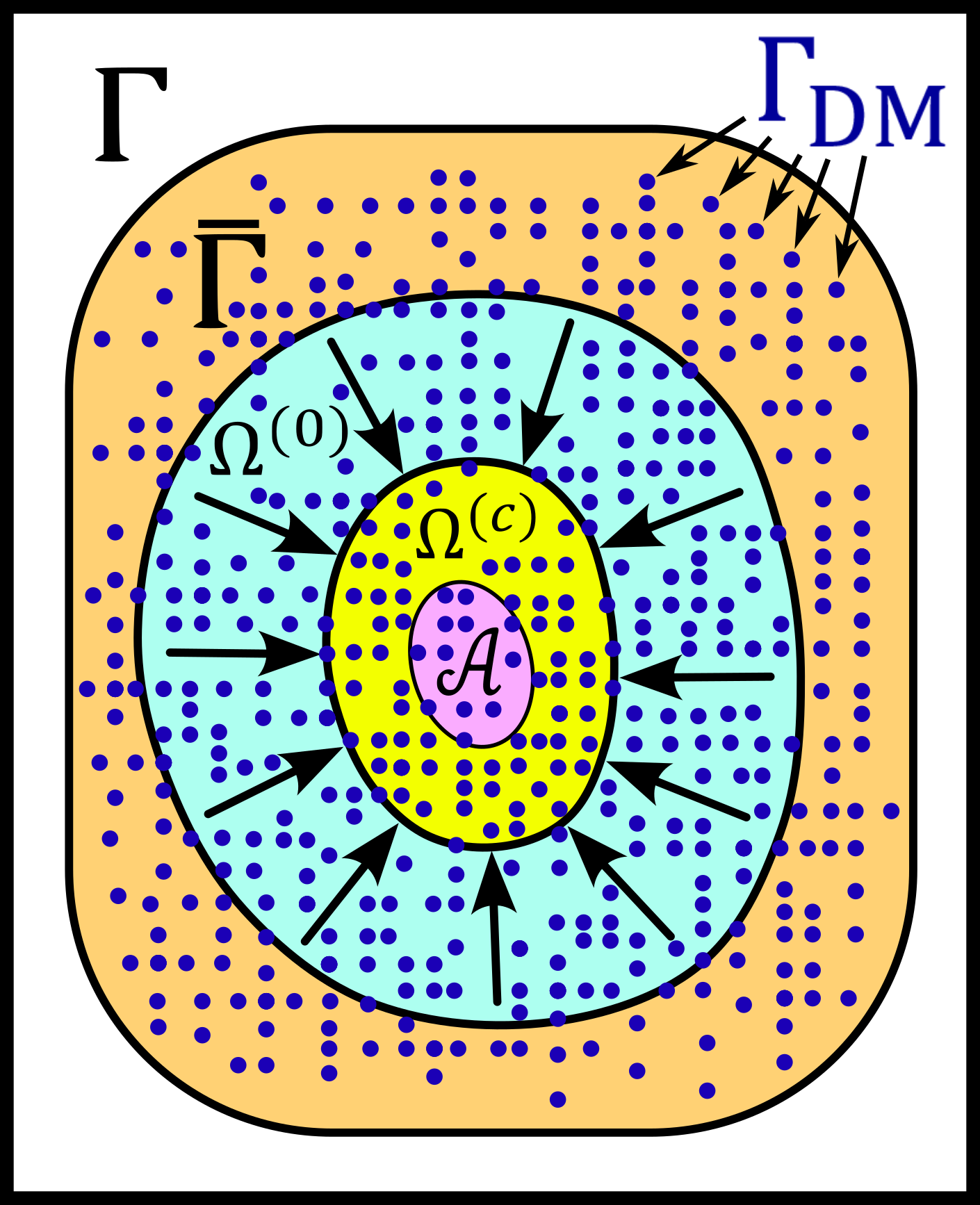
Since the DM is the part of the computer where the state \(\omega\) is written, it follows that each state of the DM correspond to exactly one \(\omega \in \Gamma\). We will write \(\Gamma_{DM}\) the finite subset of phase space that contains all possible states of the DM. The finite set \(\Gamma_{DM}\) is thus a proper subset of the phase space \(\Gamma\).
We will furthermore define the set \(\bar{\Gamma}\) to be a compact, proper closed convex subset of \(\Gamma\) which contains \(\Gamma_{DM}\). We will think of \(\bar{\Gamma}\) as a set that is just a bit larger than the smallest compact closed convex set that contains \(\Gamma_{DM}\). By “just a bit larger” we want to mean that we allow a minimal “security” distance between the boundary of \(\bar{\Gamma}\) and every element of \(\Gamma_{DM}\).
By the definition of \(\omega^{(0)}\), it is reasonable to set the restriction
We can then say informally that \(\bar{\Gamma}\) is the compact set where everything happens, so that we don’t have to care about the huge set \(\Gamma\). For any set \(\Omega \subset \bar{\Gamma}\) we systematically write its intersection with \(\Gamma_{DM}\) as
The situation is summarized in the following figure.
We now define the measure \(\nu\) on the \(\sigma\)-algebra \(\mathcal{L}\left(\bar{\Gamma}\right)\) as follows. For a given set \(\Omega \in \bar{\Gamma}\) we count the number of memory states that \(\Omega\) contains and we define it to be \(\nu \left( \Omega\right)\):
where “#” returns the cardinality of a set. One can check as an exercises that is in fact define a measure.
The measure \(\nu\) allows to define the measure space \(\left(\bar{\Gamma}, \mathcal{L}\left(\bar{\Gamma}\right), \nu\right)\). In order to work with the same set \(\bar{\Gamma}\) and the same \(\sigma\)-algebra \(\mathcal{L}\left(\bar{\Gamma}\right)\) for all measures, we extend the above introduced measure \(\tilde{\mu}^{(0)}\) over \(\bar{\Gamma}\) by defining
for all \(\Omega \in \bar{\Gamma}\). It follows that the \(\tilde{\mu}^{(0)}\) measure of any set that does not intersect \(\Omega^{(0)}\) is zero. The PDF \(p_{\tilde{\mu}^{(0)}}\) can be extended from \(\Omega^{(0)}\) to \(\bar{\Gamma}\) by setting it equal to \(0\) for any state outside \(\Omega^{(0)}\).
Since we defined a measure \(\nu\), there exist the temptation to work with its distribution function, but such a function does not exist unfortunately. The best we can think of as a density function for \(\nu\) could be
where \(B_{\epsilon}(\omega)\) is the open ball of radius \(\epsilon\) centered in \(\omega\). This function defines a measure \(\tilde{\nu}\) on \(\bar{\Gamma}\) by
Although the function \(f_{\tilde{\nu}}\) is interesting from a theoretical point of view, it leads only an approximation of \(\nu\). In the following, we will work with \(\nu\) and we will not need \(\tilde{\nu}\).
We note finally that the measure \(\nu \left(\Omega\right)\) is linked to the number of bit that are needed to encode all states of the memory that are in \(\Omega\). Since \(\nu \left(\Omega\right)\) is the number of such states, we can write the number of bits needed to encode them as
It follows from that definition that
If we now start the iterative algorithm by an initial guess in the set \(\Omega^{(0)}\) and iterate the map \(\Phi\) until \(\Omega^{(0)}\) is compressed to \(\Omega^{(c)}\), the number of bits needed to encode all states in \(\Omega^{(0)}\) shrinks to the number of bits needed to encode all states in \(\Omega^{(c)}\). This reduction of needed number of bits is
Rewriting this reduction of bit number as \(\Delta B^{(c)}\) we get
In the next sub-section, we will define the information gain \(\Delta I^{(c)}\) associated to the compression of \(\Omega^{(0)}\) to \(\Omega^{(c)}\) as
It follows from those definition that the relation between the reduction of bit number and information gain is
In the discussion sub-section, we will argument that Landauer’s erasure can be re-interpreted as this reduction of bit number.
The Heat Engine
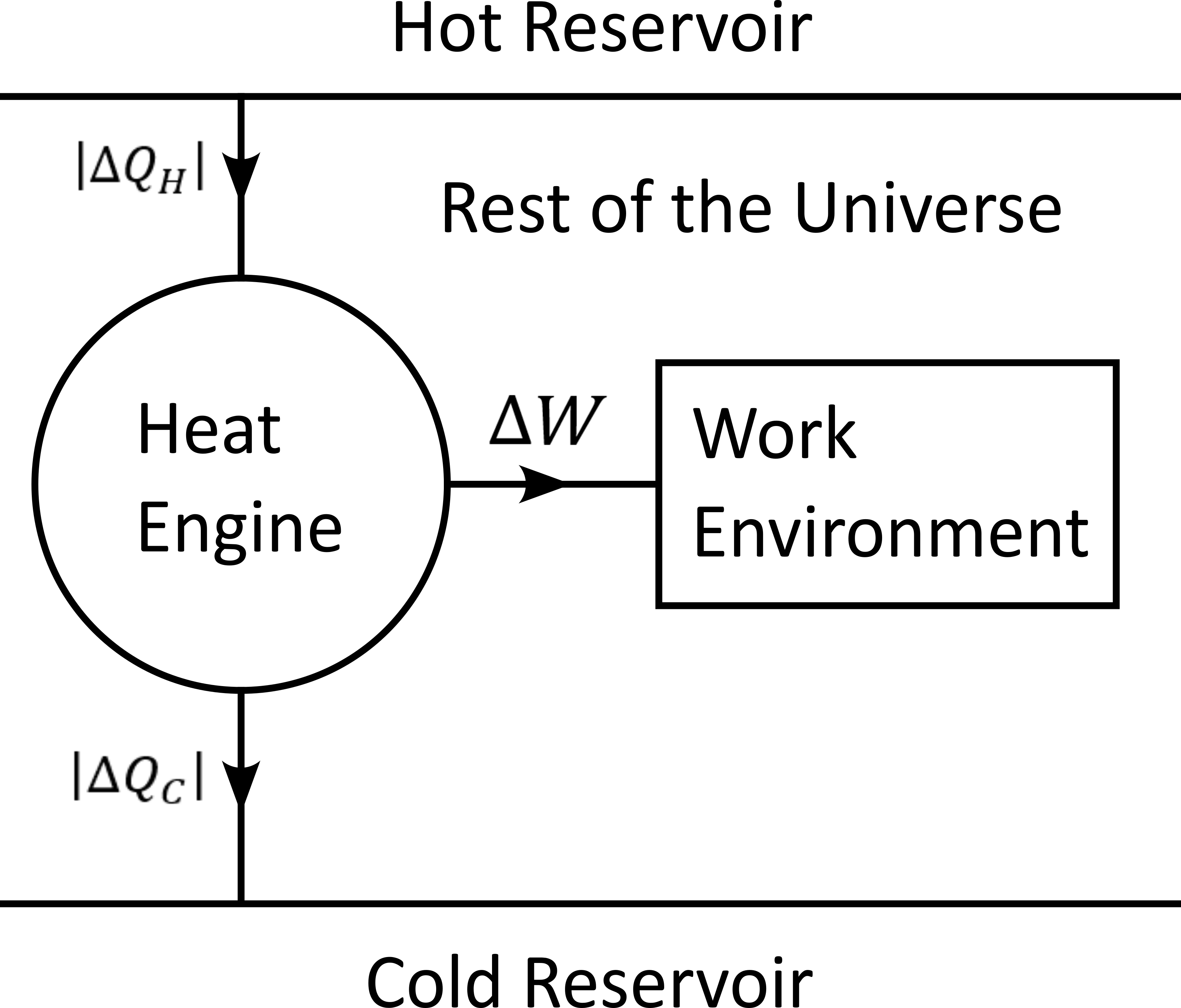
Work is the useful thing that a heat engine gives to some part of the universe that we will call the work environment. Although this “work environment” is usually not part of the thermodynamic descriptions, there is nothing wrong about it: it is just the part of the universe the heat engine is acting on. This notion will appear to be convenient for the rest of the text. The heat engine performs some work in the work environment by transferring heat from a hot to a cold reservoir. The heat engine and the working environment are two subsystems and the hot reservoir, cold reservoir and the rest of the universe are three other subsystems. Their union being the universe (the total system).
The heat engine operates in a cyclic way so that its state is the same at the beginning of each new cycle. In contrast, the states of the work environment, the rest of the universe and the heat reservoirs can evolve along the cycles. The goal of a heat engine is in fact to transform the work environment, else the engine would be useless. The transformation of the work environment often translates in a lowering of its entropy, while the entropy of the rest of the universe together with the heat reservoirs is increasing. The transformation is reversible exactly if the entropy of the universe (total system) remains constant during that transformation. If the transformation is irreversible, the entropy of the universe increases, even if entropy of the work environment decreases. Since the entropy is a function of state, the entropy of the heat engine is the same at the beginning (and end) of each cycle.
For the coming comparison between a computer and a heat engine, we would like to focus on the special case described in the following figure.
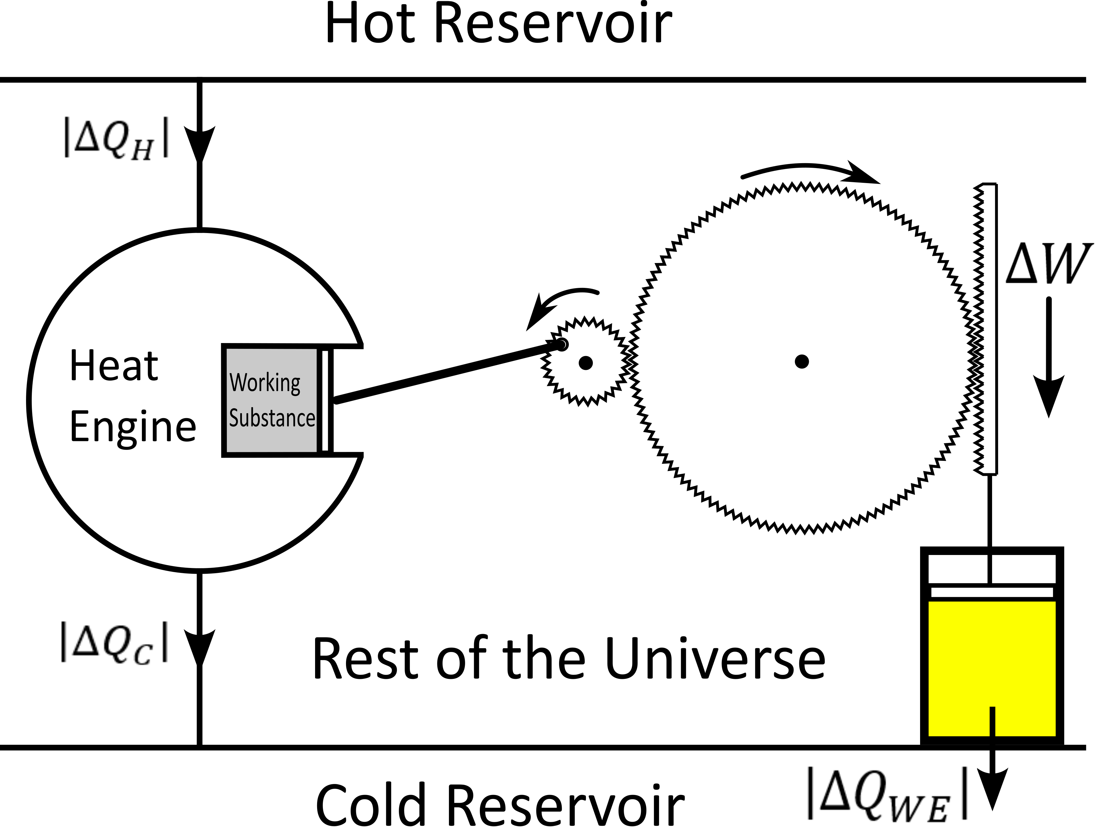
It represents a heat engine that gives energy to a working environment (WE) in the form of a mechanical work amount \(\Delta W\). This work is used to compress an ideal gas in a cylinder in thermal contact with the cold reservoir at temperature \(T_C\). In order to be able to evaluate entropy changes, we admit that no irreversible loss of energy happens. This means that the heat engine is an ideal (reversible) heat engine, which is called a Carnot engine. It has therefore maximal efficiency. We also have to assume that the gas compression is isothermal, which means that the movement has to be sufficiently slow as guaranteed by the coupling of the small and large wheels. We admit that there is a good isolation between the rest of the universe and to two subsystems implied in the process, which are the heat engine and the WE. A flow of energy travels through the subsystem made of the pair heat-engine + WE. At each cycle of the engine, a heat amount
enters that subsystem and a heat amount
leaves that sub system. Since the temperature of the gas in the WE do not changes, its internal energy do not change as well. That means that the work \(\Delta W\) is equal to the expelled heat amount \(\lvert \Delta Q_{WE} \rvert\). The conservation of energy reads thus:
The volume of the ideal gaz is decreased by an amount \(\lvert \Delta V \rvert\) at each cycle. We will write \(V > 0\) the volume of the ideal gaz at the current cycle. The change of entropy \(\lvert \Delta S_{WE} \rvert\) is therefore negative and given by
where \(N\) is the number of particle of the ideal gas and \(k_B\) is the Boltzmann constant.
During one cycle, the hot reservoir experiences a drop of entropy by an amount
while the cold reservoir experiences a grow of entropy by an amount
Since the engine comes back to the same state after every cycle and since entropy is a function of state, there is no change of entropy in the engine after each cycle. Assuming the process to be reversible, the total entropy is conserved:
If the process is now irreversible (like any realistic, non-ideal process), the entropy drop in the ideal gas will still be the same since the entropy is a function of state, but the heat exchanges will be different and this will lead to a positive entropy grow of the universe (the total system) by the second law of thermodynamic, even if entropy was locally decreased in the ideal gas:
where the subscript \(Rest\) refers to the rest of the universe.
This scheme of producing an energy flow through a system in order to drain out some of its entropy (a side effect being an entropy grow of the universe) is a general scheme encountered everywhere in engineering and nature. Plants and animal do that all the time. We eat energy to produce mechanical work such as moving from a place to the other, but a large part of the energy we eat is expelled as thermal radiation associated to a drop of our entropy. In fact, our body continuously experiences injuries because chance unbuild things more often that it builds it. Those injuries are structural changes that have a high probability to happen by chance alone and which correspond to an increase of entropy of our body. Because of injuries, the entropy of our body tends to increase. In order to survive, we have to consume energy to continuously put our body back to order i.e. to a state that has very little chance to be reached by chance a lone, that is, a state a low entropy. Repairing our body implies thus to consume energy to lower our entropy back to an organized state and that implies to expel an associated amount of heat by radiation. This scheme is so universal that we will now try to apply it to computers in order to build an analogy with the eat engine. We will try that way to deduce a definition of thermodynamical quantities in the context of iterative algorithms.
The Computer as an Engine
Here are a few empirically facts. If the reader does not agree with them, just consider that they are assumptions. We assume furthermore that the iterative reconstruction in question is correctly implemented.
Given a converging iterative reconstruction for some given data, the image quality along iterations improves then monotonically, at least in average in some temporal window.
Each iteration of an iterative reconstruction consumes electric power and time, the product of both (or time integral of power) being the energy consumed by that iteration.
An image, together with the other dynamic variables of the algorithm, is physically a state of the dynamic memory. A converging reconstruction process is a process that changes the state of that memory until the resulting state do not longer significantly changes.
During an iterative reconstruction process, if the reconstructed image improves and converges (at least in average in some temporal window), the computer absorbs electrical energy, a part of that energy serves to set its memory in a certain state, and most of the absorbed energy is released in the environment as heat.
A reconstructed image of good quality is an image that models the measured data reasonably well (relative to a given model), and which satisfies some prior knowledge reasonably well. Both criteria result in a low value of the objective function if that function exist.
An image of good quality corresponds to some states of the dynamic memory that have very little chance to be found by chance alone, for example by a random search for a good image.
It is not the intention of the author to build some axioms of a mathematical theory. The empirical facts above are in fact redundant to some extends, but we don’t really care. We just want to build an intuition for a thermodynamic theory of MRI reconstruction.
The intuition following from those fact is that the computer consumes energy to set its memory in a state of low entropy, and that those states of low entropy are the element of the attractor of the algorithm i.e. the elements that are solution of the problem our iterative algorithm is solving. It is intuitively clear that an iteration that moves the current state \(\omega\) towards the attractor (and thus lower the entropy of the memory) must consume energy, but the reverse does however not need to be true: more energy consumption does not need to lead to an image quality gain, since energy can be directly dissipated into heat. A notion of efficiency is therefore missing and there is no obvious definition for it. Intuitively, it makes sense to define efficiency in such a way that it expresses a gain in the result quality related in some way to the energy consumed for that gain. But there is no obvious definition for that efficiency.
Instead of trying to force a definition, we propose to develop a thermodynamic theory of the computer in order identify what could be the natural notion for thermodynamical quantities in that context. We will build a “computer engine” in analogy to the heat engine in order to inherit some notions from thermodynamic to the context of information and algorithms. We will then propose some definition of efficiency, thermodynamical entropy, information theoretical entropy and information along the way.
During an algorithm is running, electrical energy given to the computer and is expelled as heat in the cooling system, which may be interpreted as the cold reservoir. In order to make an analogy between the computer and the heat engine, we define the following virtual partition of the universe:
the electric power supply system (PS), which transfers energy to the computer,
the computer (Comp), with the computational units and including the part of memory that contains the program, but without the part of memory that contains the dynamic variables of the reconstruction process,
the part of memory that contains the dynamic variable of the reconstruction process, that we will call the dynamic memory (DM).
the cooling system (C) of the computer.
the rest of the universe, which also absorb parts of the heat released by the computer.
Note that the union of these five parts is the universe.
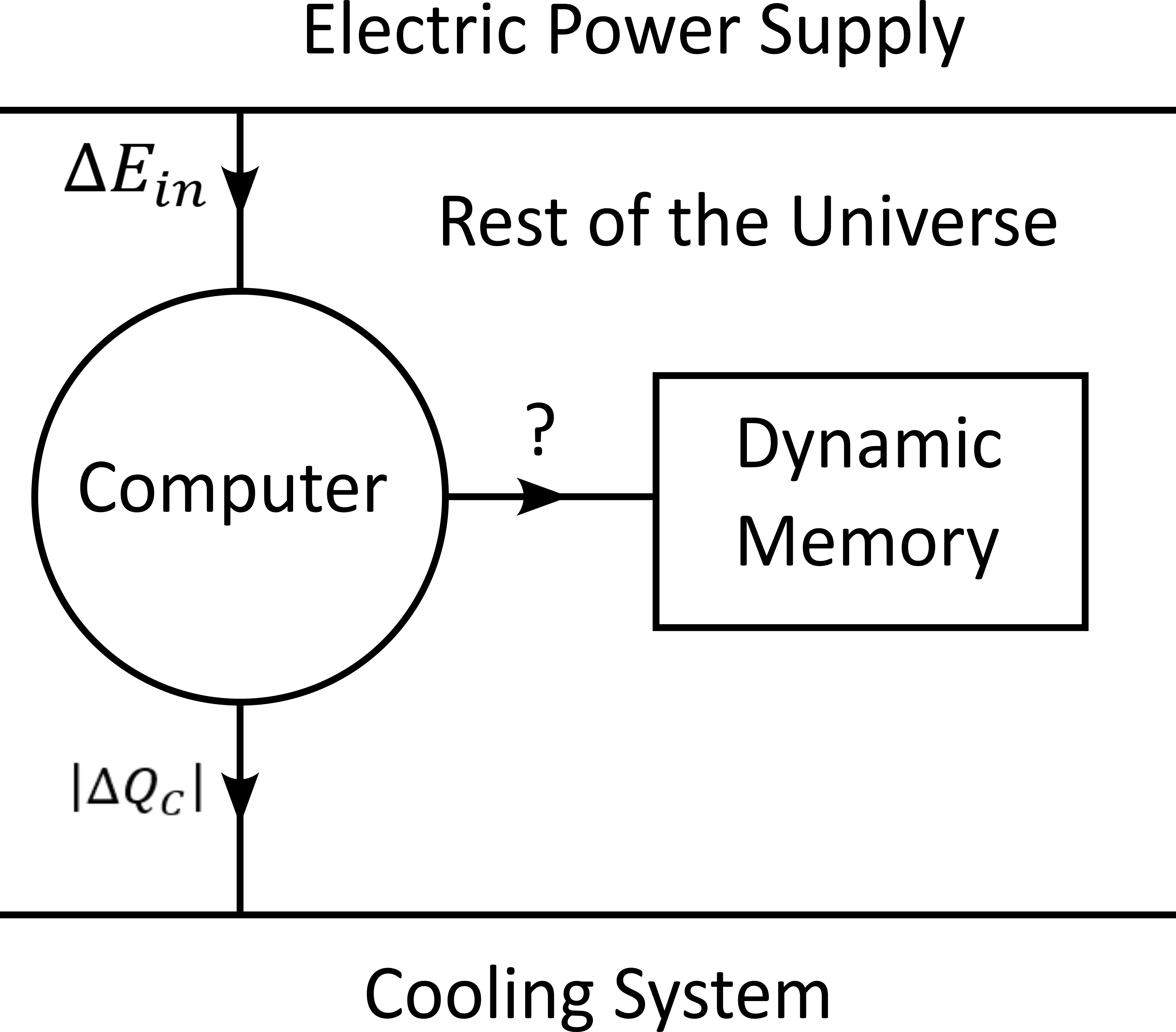
A very important fact about our description is that the dynamic memory (DM) is considered to be out of the computer, which was not explicitly stated until now in our description. It means that the DM is virtually separated from the rest of the computer in our virtual separation of the universe in subsystems. The DM is the analog of the working environment for the heat engine.
We propose here to consider the computer as an engine and to interpret one iteration of the reconstruction process as one cycle of the engine. In fact, at the beginning of each iteration, the state of the computer is the same since we consider all changing (dynamic) variables to be in the DM, which is the analog of the work environment of the heat engine. The energy given to the computer is almost completely dissipated into heat transmitted to the cooling system at temperature \(T_C\). We neglect transmission of heat given to the rest of the universe because it should be much smaller. Also, there are some electro-magnetic radiations emitted from to the computer to the rest of the universe and some electrostatic energy that is stored in the memory, since writing information in it implies to set a certain configuration of charges with the associated electro-static energy. These two energy amounts are however so small as compared to the energy dissipated in the cooling system that we will neglect them. As a consequence of energy conservation, we will therefore write for one cycle
That means that all the energy entering the computer is dissipated as heat in the cooling system. Following the intuition that this flow of energy drains out some (thermodynamical) entropy from the dynamic memory (DM) as it brings it in a state that can hardly be reached by chance alone, we expect that a negative entropy change \(-\lvert \Delta S_{DM} \rvert\) is produced in the DM during one cycle (one iteration) of the MRI reconstruction process. If our intuition is correct, the second law of thermodynamic implies then
where equality holds for a reversible process. But the quantities \(\Delta S_{DM}\) and \(\Delta Q_C\) are signed in that expression. Assuming \(\Delta S_{DM}\) to be negative, we deduce
Since the computer is in the same state at the beginning of each iteration, it experiences no entropy change between each start of a new iteration. The entropy change in the system computer + DM is therefore to be attributed to the entropy change in the DM only. The previous inequation means that for an entropy drop of magnitude \(\lvert \Delta S_{DM} \rvert\) in the DM, there must be a heat amount of magnitude at least \(T_C \lvert \Delta S_{DM} \rvert\) expelled to the cooling system. We will write \(E^{tot}\) the total amount of energy given to the computer for the reconstruction and \(\lvert \Delta S_{DM}^{tot} \rvert\) the magnitude of the total entropy drop in the DM during reconstruction. It follows from the previous equation, from our formula for energy conservation and from the fact the temperature of the cooling system is constant, that
If we express \(E^{tot}\) as the multiplication of the input electric power \(P\) and the total reconstruction time \(\Delta t^{tot}\), we get
If we can find a way to establish the magnitude of the total entropy drop in the DM associated to a desired quality of result, for a known electric power, we could then deduce a minimal reconstruction time for the desired MRI quality.
We have done a first analysis of what could be a computer engine by formulating the first and second law of thermodynamic for the chosen virtual partition of universe. The analogy between the computer and the heat engine is however limited because we are for the moment unable to define what the computer is transmitting to the DM, as pointed out by the quotation mark in the last figure. The reason is that the computer performs no mechanical work and we have to find a replacement for work in order to continue the analogy. We implement a solution to the problem in the next subsection.
A Postulate for the Thermodynamical Entropy of the Dynamic Memory
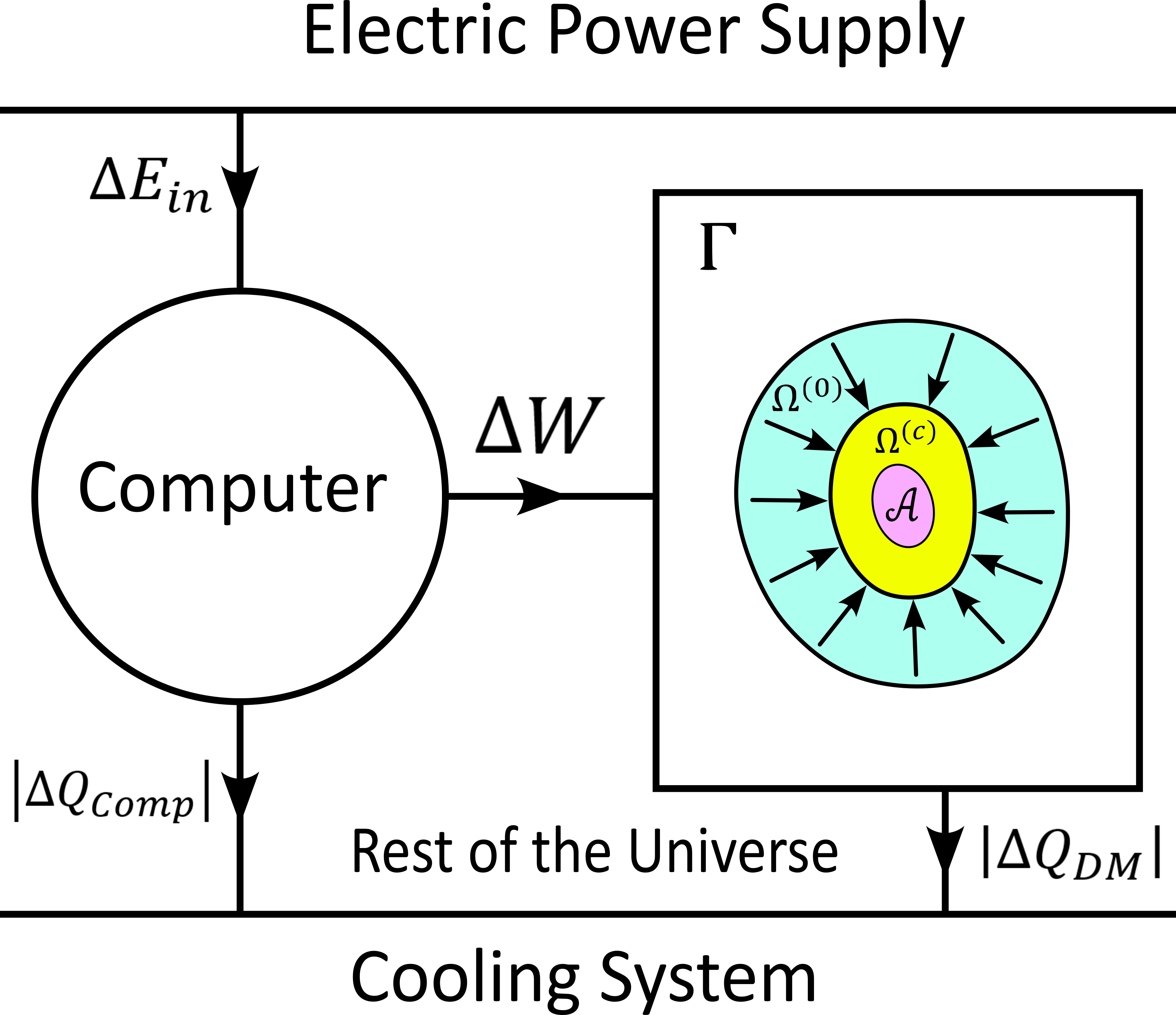
We propose to solve our difficulties by the following heuristic (actually quite esoterique) construction. Instead of considering that the computer interacts with the dynamic memory, we consider that nature is as if the computer was interacting with the phase space. The variables stored in the DM represents one state in the phase space, but since it could be any, the computer behaves in a way that would do the job for any state in the phase space. We consider therefore that it is a reasonable argument to say that the behavior of the computer is related phase space and not related one particular representant. The computer behaves as if it was reconstructing many MRI images at the same time. Instead of discussing endlessly how realistic or not that argumentation is, we propose here one implementation of that idea and we will pragmatically try to see what are the implications.
In analogy to the isothermal compression of an ideal gas, we will consider that the computer is compressing a portion \(\Omega^{(0)}\) of phase space by iterating the map \(\Phi\) that dictates the evolution of the iterative MRI reconstruction algorithm. We chose \(\Omega^{(0)}\) to be the region of phase space where there is a non-zero probability that our initial value \(\omega^{(0)}\) is chosen. For convenience, we will like to think of \(\Omega^{(0)}\) as a proper closed convex set. We recall that it contains the attractor \(\mathcal{A}\) of the dynamical system. We define the set
We imagine that \(\Omega^{(c)}\) is the set \(\Omega^{(0)}\) compressed by \(\Phi\) after \((c)\) iterations. We imagine that \(\Omega^{(c)}\) contains an ideal phase space gas and that at each iteration, a part of the energy given to the computer is transformed in a kind of informatic work \(\Delta W\) to compress that phase space gas. We will therefore call \(\Omega^{(c)}\) the compressed set at iteration \(c\). The situation is described in the following figure.
We will imagine that any connected proper subsest \(\Omega\) of phase space with non-zero Lebesgue measure contains a certain amount of our “phase space ideal gas”. Inspired by the equation that describes an ideal gas with constant temperature \(T_C\), we set
where \(p\) is the pressure of our phase space gas, \(V\) is its volume given by the measure \(\nu\) as
and \(k_{\Gamma}\) is the ideal gas constant of our phase space gas. It follows that
We deduce that the work \(\Delta W\) needed to compress \(\Omega\) to a smaller subset is \(\Omega'\) is
We will now label some quantities with the super-script \((c, c+1)\) to indicate that the quantity in question is associated to the iteration number \((c)\), which performs the transition from state \((c)\) to state \((c+1)\). We will also label a quantity with super-script \((c)\) in order to indicate that this quantity is associated to the transition from the initial state to the state number \((c)\).
We can now express the conservation of energy (the first law of thermodynamic) as follows. An energy amount \(\Delta E_{in}^{(c, c+1)}\) is given to the computer, an amount \(\Delta E_{in}^{(c, c+1)} - \Delta W^{(c, c+1)}\) is dissipated to the cooling system by the computation at temperature \(T_C\), and another amount \(\Delta W^{(c, c+1)}\) is given as work to the phase space and then also dissipated to the cooling system as a heat amount \(\lvert Q_{DM}^{(c, c+1)} \rvert\) at temperature \(T_C\). It holds thus
and we define
the heat amount dissipated by the computation directly to the cooling system. This is the part of the energy that is not “transmitted” to the phase space. The conservation of energy can then be rewritten as
Of course, the phase space is a mathematical, non-physical object and the work given to phase space is a symbolic language. What we try to do is an intellectual effort that consists in admitting that nature behaves as if the computer was in fact transmitting work to the phase space.
From analogy of phase space with an ideal gas, we postulate that the (physical) thermodynamical entropy drop in the DM during iteration number \((c+1)\) is
The total entropy drop due to all iterations until (and with) iteration number \((c)\) is therefore
and thus
Our postulate for the entropy change of the DM can also be express from state \(0\) to state \(c\) as
Assuming that DM and cooling system are in thermal equilibrium, the process is then reversible and the second law of thermodynamic implies
This is consistent with a reversible isothermal compression of an ideal gas, as assumed. We will assume that the rest of the universe experiences no heat exchange during a reversible process so that the entropy of that part is unchanged. Since the computer is a cyclic engine, it is also experiencing no changes of entropy between the beginning or each new cycle. The non-zero entropy changes during the reversible process are therefore those of the power supply system \(\Delta S^{(c, c+1)}_{PS}\), of the cooling system \(\Delta S^{(c, c+1)}_{C}\), and of the DM written \(\Delta S^{(c, c+1)}_{DM}\). For a reversible transformation holds thus
The entropy change of the cooling system can be evaluated as
By substitution of the above formulas holds
This is the expression of second law for the total system in the case of a reversible process. If the process is not reversible (as any realistic process) we expect inequations instead of the equations above. For the dynamic memory, the second laws for an irreversible heat transfer implies
For the cooling system, the second law implies
For the power supply system, we simply assume that the second law implies
and similarly for the rest of the universe
Where the subscript \(Rest\) refers to the rest of the universe. As mentioned above, the entropy change of the computer over one cycle is zero. The entropy change for the total system reads then
We have thus formulated the first law for the total system as well as the second low for the total system in the case of a reversible process and an irreversible process.
The key notion introduced in the present subsection is a postulate for the physical, thermodynamical entropy of the DM. We postulate that the physical entropy drop in the DM can be described in term of a mathematical compression of \(\Omega^{(0)}\) instead of physical quantities.
Information and Efficiency
For the coming comparison with information theory in the next subsection, we define the information gain associated the transition from \(\Omega^{(c)}\) to \(\Omega^{(c+1)}\) as
We define as well the gain of information associated to all iterations until (and with) iteration number \(c\) as
it follows
By our postulate for the entropy change in the dynamic memory, and by our definition of information gain it holds
We get then a relation between physical work (in Joule J) and information, for iteration number \({c+1}\), given by
Alternatively, for all iteration until (and with) iteration number \({c}\), we obtain
It follows in particular from these last two equations that, whatever the unit of information is, the constant \(k_{\Gamma}\) must have the unit J/K/[Unit of Information]. We are now able to define a notion of efficiency \(\eta^{(c, c+1)}\) as the ratio of the input energy \(\Delta E_{in}^{(c, c+1)}\) (during one cycle) and the work performed on the phase space \(\Delta W^{(c, c+1)}\):
If we admit that the DM experiences an entropy drop of magnitude \(\lvert \Delta S^{(c, c+1)}_{DM} \rvert\) during one iteration. We deduce from (E3) that
If the efficiency is constantly equal to a number \(\eta\), summing up all contribution of the entire reconstruction duration leads
which is a more severe constraint on the entropy drop of the DM as compared to the one we got earlier. It follows in particular that
This inequation is the main result of our theory. We will see in a next section that it is actually equivalent to Landauer’s principle if we set \(k_{\Gamma}\) equal to the Boltzmann constant. We will also deduce a new interpretation of Landauer’s erasure in term of bit number reduction needed to encode the states in the compressed set.
Connection with the Theory of Information
In the previous subsection, we introduced some relation between the physical energy E and the thermodynamical entropy S as well as a notion of information I with some relation to E and S.
In this section, we will introduce some relations that relates the thermodynamical entropy S to the information theoretical entropy H. The entropy H is always defined on a probability distribution while we defined an entropy notion S for some subset \(\Omega\) of the phase space \(\Gamma\). The simplest way to relate them is to define a probability function for any given subset \(\Omega \subset \Gamma\). We proceed as follows.
Since \(\Gamma_{DM}\) is a finite set, we will call \(nDM\) its cardinality. It is the number of states that can be stored in the dynamic memory. Let be \(\omega_i\), the element number \(i\) in \(\Gamma_{DM}\), where \(i\) runs from \(1\) to \(nDM\). For a given subset \(\Omega \subset \Gamma\), we define the probability \(p_i\) for \(\omega_i \in \Gamma_{DM}\) as
This assigns to each \(\Omega \subset \Gamma\) a probability distribution on the set \(\Gamma_{DM}\). We can then evaluate its entropy H as
and therefore
Since this entropy is associated with the set \(\Omega\), we will write it \(H \left(\Omega\right)\). We now identify \(\Omega\) with the compression of \(\Omega^{(0)}\) by \(c\) iterations, which is the set \(\Omega^{(c)}\). The associated information theoretical entropy is then
We define the change of information theoretical entropy \(\Delta H^{(c)}\) as
By definition of the information gain \(\Delta I^{(c)}\), the (thermodinamical) entropy change of the DM \(\Delta S_{DM}^{(c)}\), and the number of bit reduction \(\Delta B^{(c)}\), we obtain
If our definition are well chosen, these four notions are, up to a factor, different names for the same thing.
Parallel Computing
We redefine in this section our notion of entropy change \(\Delta S\), information theoretical entropy change \(\Delta H\), information gain \(\Delta I\), and number of bit reduction \(\Delta B\) in the case of \(N\) copies of the dynamic memory being updated in parallel by the same iterative algorithm. In this context, each copy of the dynamic memory is storing its own dynamic variable independently of each other. The \(N\) copies of the dynamic memory are physically different memory storage systems that are physically very identical, which are informatically identical, but which all have their individual existence. We will write \(\omega_i\) the dynamic variable stored in the dynamic memory number \(i\). Each \(\omega_i\) can be different from the others and they are all independent.
In order to describe that system, we define a new single state \(\omega\) as the list
in the new phase space
which obeys to all definition we did until now. We only have to replace \(\Gamma\) by \(\Gamma^N\) and \(\omega\) by \(\left(\omega_1, ..., \omega_N \right)\) in all our definitions.
We will ow do that but we will keep the same definition for \(\Omega^{(0)}\) and \(\Omega^{(c)}\) as above. Since the algorithm is behaving in the same way irrespectively of the particular state of each dynamic memory, the set \(\Omega^{(0)}\) is the same for all DMs and so is the set \(\Omega^{(c)}\). Only the particular representant \(\omega_i\) can differ between DMs. The start value \(\omega^{(0)}\) is in the set \({\Omega^{(0)}}^N\) and the state \(\omega^{(c)}\) at iteration \((c)\) is in the set \({\Omega^{(c)}}^N\) given by
In that expression, we silently redefined \(\Phi\) on \(\omega \in \Gamma^N\) component wise by
For a subset \(\Omega \subset \Gamma\), the number of states in \({\Omega}^N \subset {\Gamma}^N\) is simply \({\nu \left(\Omega\right)}^N\). That means
By our definition of the entropy change \(\Delta S^{(c)}\), the compression from \({\Omega^{(0)}}^N\) to \({\Omega^{(c)}}^N\) corresponds to an entropy change
In a similar way, we deduce that the work to perform that compression is given by
Since the informatic work \(\Delta W\) to perform the set compression is equal, by our assumption, to the heat released by the dynamic memory, it follows that this heat amount is also multiplied by \(N\) for the parallel execution of the algorithm on \(N\) dynamic variables.
The definitions of \(\Delta I\), \(\Delta H\) and \(\Delta B\) are equal to \(\Delta S\) up to a constant, they are also all multiplied by \(N\) for the parallel computing. We conserve thus the relation
We note finally that the work \(\Delta W\) is the mechanical work that would be needed to compress a gas verifying the law
which is similar, up to the constant \(k_{\Gamma}\), to the ideal gas law. The formulas are as if the \(N\) independent dynamical variables \(\left(\omega_1, ..., \omega_N \right)\) were living in the same volume inside phase space \(\Gamma\) in a similar way like \(N\) particles of an ideal gas are evolving in the same physical volume without interacting between each other.
Connection with the Landauer’s Principle
By writing the total consumed energy as \(\Delta E^{tot}\), and by writing the temperature \(T_C\) as \(T\) (which is the temperature at which the computer operates), equation (E5) can be rewritten as
This equation is very similar to the principle of Landauer, which reads
where \(k_{B}\) is the Boltzmann constant, \(T\) is the temperature of the computer and \(\Delta E\) is the practical energy amount that is needed to erase a bit of information. Since Landauer’s principle is formulated “per bit”, we can write it more generally for \(\Delta B\) bits as
where \(\Delta E\) is now the energy needed to erase \(\Delta B_{erased}\) bits. If we substitute \(\Delta I^{tot}\) by the equivalent expression for the number of bit reduction \(\Delta B\), equation (E7) becomes
which is now very close to Landauer’s principle. The main difference is the presence of constant \(k_{\Gamma}\) instead of \(k_B\). This suggests to set
Equation E9 becomes then
By interpreting the useful energy \(\eta \ E^{tot}\) as being \(\Delta E\), and by interpreting the number of erased bits \(\Delta B_{erased}\) as the number of bit reduction \(\Delta B\) in the context of iterative algorithms, Landauer’s principle E8 is equivalent to E10, which is the equation that follows from our postulate for the change of entropy in the dynamic memory. We have thus demonstrated that our postulate for the entropy of the dynamic memory leads to an expression that can be interpreted to be to Landauer’s principle extended to the iterative algorithms.
Given the temperature dependency of E8 and E10, which is so that the information gain explodes when temperature is going to \(0\), it is natural to wonder weather these equations could be the classical limit of a quantum equation, since the nature of quantum computing is to exploit the properties of matter for very low temperature. Although it is purely speculative, it may then be that the number of particles \(N\) becomes the number of dynamic variables that are existing in parallel in the quantum algorithm.
Connection with Statistical Mechanic
The entropy of an ideal gas, for a constant number of particles \(N\) and constant temperature, can be expressed up to a constant as
An analogy with our ideal phase space gas and equation (E6) suggests, for the entropy of the dynamic memory, an expression of the form:
Neglecting the constant leads
The Boltzmann entropy formula reads
where \(\Omega\) is the area of the surface in phase space occupied by all the possible micro states of a given energy for the physical system under consideration (it is the “number” of allowed micro-states, if one prefers). Both entropy formula are very similar because the meaning of \(\Omega\) in Boltzmann formula has a similar meaning like the symbol \(\nu \left({\Omega}^N\right)\) : it is the number of states that the system under consideration can occupy.
It seems therefore that a connection between our theory with statistical mechanic may be possible. But for the moment both theories are quite different, mainly because our notion is volume is equal to the number of states that DM can occupy, while in statistical mechanic are volume and number of possible states different notions. A unification will therefore need a work of reformulation.
Artificial Intelligence as an Amplification of Efficiency
We will not speculate of what artificial intelligence (AI) could be in the future and what it could achieve potentially. Rather, we will consider it as what it is for the moment in the context of MRI reconstruction: artificial intelligence in MRI reconstruction consists in replacing the evaluation of some dynamical variable (image, deformation field or other algorithm variable) by some statistical prediction that are faster to perform if the model could be trained in advance on some good quality ground truth data.
For the moment, it seems therefore that the use of AI allows the same gain of information as the non AI algorithms but in a smaller amount of time, and therefore by consuming less energy. It may seem at first sight that AI can allow to violate some lower energy bound set some physical principle, such as Landauer’s principle. But if we think that training an AI consumes actually a large amount of energy and that the data the AI is trained on also needs a large energy amount to be reconstructed, it becomes clear that a careful sum of all energy contributions must be done in order to perform a correct analysis.
We will call \(E \left(GT\right)\) the energy amount needed to produce the data that serves to train the AI (“GT” stands for “ground truth”) and we will call \(E \left(\mathcal{N}\right)\) the energy needed to train the statistical model (i.e. the AI). We will write \(E_i\) the energy needed to perform a non AI algorithm on data number \(i\) in order to obtain a certain quality in the result. Finally, we will write \(E^{AI}_i\) the energy needed by an AI informed algorithm that leads to the same quality of its non AI counterpart for data number \(i\). We run now \(R\) times the non AI algorithm on \(R\) different data. The total consumed energy is therefore
If we run the AI informed algorithms on the same data until the same quality of result is obtained, the total consumed energy is
The assumption that the AI reconstruction consumes less energy that its non AI counterpart reads
For a large enough \(R\) we can then reach
This means that the initial energy investment \(E \left(GT\right) + E \left(\mathcal{N}\right)\) becomes valuable for sufficiently many reconstructions.
We will call \(\langle E \rangle\) the average energy consumption of the non AI algorithm so that
and will call \(\langle E^{AI} \rangle\) the average energy consumption of the AI algorithm so that
It follows that for sufficiently many run of the algorithms holds
We will write \(\Delta I^{tot}\) the total information gain of all non AI reconstruction, which is by our definitions also equal to the total information gain of all AI reconstruction. By our definition of efficiency, and assuming it to be constant for simplicity, it follows that the efficient of the non AI reconstruction is given by
and that the efficiency of the AI reconstruction is given by
Their ratio verifies
and therefore
The efficiency of the AI algorithm is then an amplification of the efficiency of the non AI algorithm. This amplification of efficiency is inherently linked to the fact that the AI reconstruction consumes less energy than the non-AI one for the same information gain. We will therefore rewrite the above relation in term of energy differences in order to highlight their implications. We define
We define their average as
We also define the initial energy investment of the AI algorithm as
We note then
A division by \(R\) leads then
For a large enough \(R\), we can therefore neglect \(E_0^{AI}\) and assume
It follows
and therefore
This situation is as if AI was a way to reuse information contained in the ground truth in order to complete the information that has to be computed to treat the supplementary data set numbered from \(1\) to \(R\). The reuse of the ground truth information requires an addition cost of energy to train a statistical model. But since this energy investment has to be done only once, it becomes valuable for a large \(R\). The situation is depicted in the following figure.
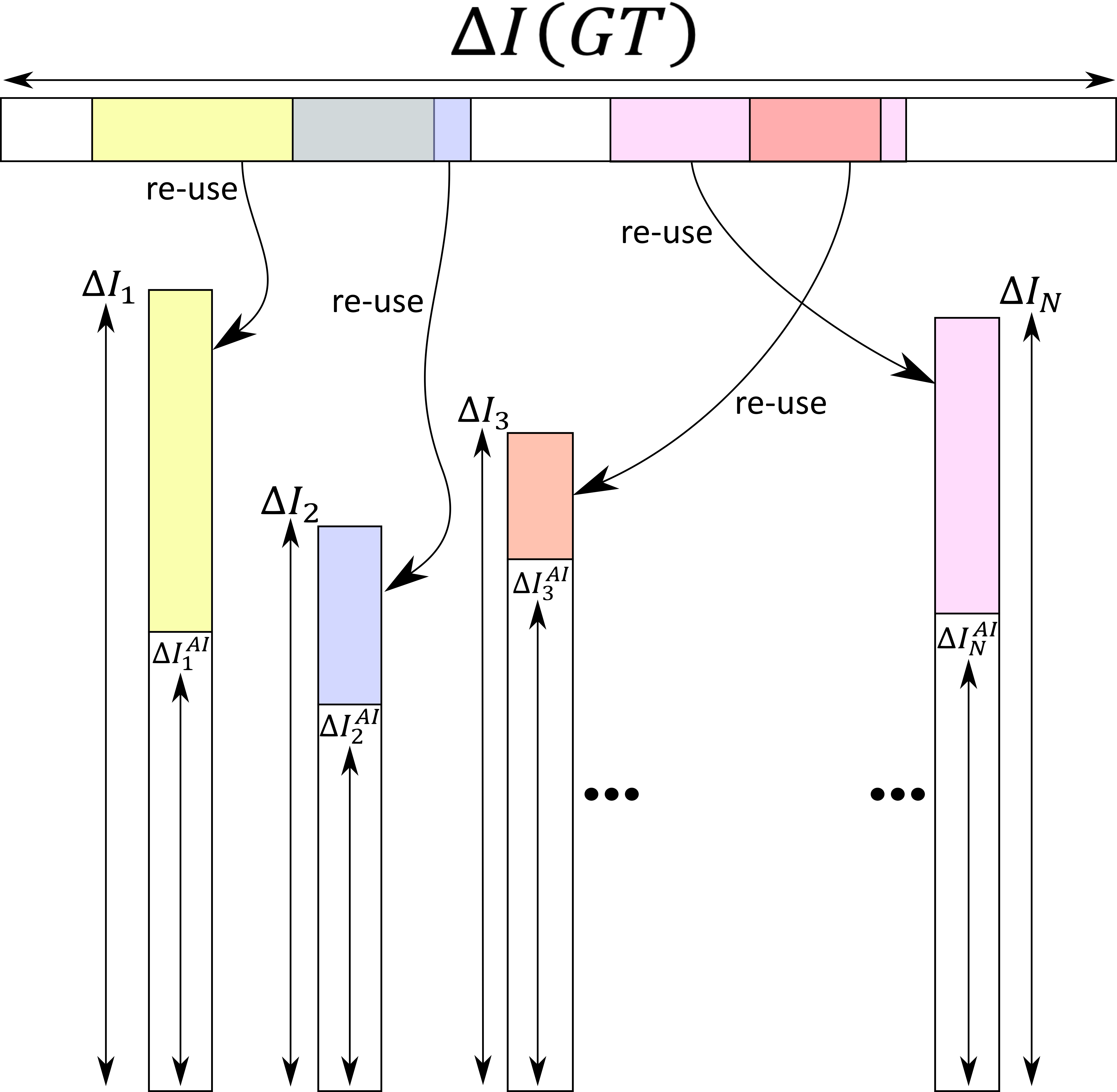
We have written \(\Delta I\left(GT\right)\) the information gained by constructing the ground truth, \(\Delta I_i\) the information gained to treat data number \(i\) with the non AI algorithm, and \(\Delta I^{AI}_i\) the information gained to treat data number \(i\) with the AI algorithm.
Conclusion
We have done two postulates on the entropy change of the Dynamic Memory (DM) of a computer (the part of memory that is changed by the iterative algorithm):
At each iteration of the algorithm, the entropy of the DM experience a negative change \(\Delta S\).
This negative change is given quantitatively by
In the second postulate is \(N\) is the number of parallel instances of the memory that the algorithm is updating (which is \(1\) for non-parallel computing), \(k_B\) is the Boltzmann constant, \({\Omega}^{(c)}\) is the phase space sub-set that contains with 100% chance the dynamic variable of any of the memory instance at iteration number \(c\), and \(\nu\left({\Omega}^{(c)}\right)\) is the number of memory state (for a single memory instance) that is contained in the phase space subset \({\Omega}^{(c)}\).
We have thus postulated some expression for the physical entropy change in the dynamic memory of a computer which rely on the mathematical dynamic variables of the algorithm rather than on some physical quantities. That way, we built a bridge between the physical word and the mathematical world of information. We did not prove that our statement for the physical entropy change in the dynamic memory was correct or wrong, but we showed that by a clever definition of information gain, our statement was very close to the known Landauer’s principle. That connection is interesting in itself.
Although less strong, we also showed some connection from our entropy postulate to the theory of information as well as to statistical mechanic.
We also showed that from our definition of efficiency follows, that the use of AI in iterative algorithms to update some of the dynamic variables at each iteration results in an efficiency amplification. In this context, AI appears like a technology that allows to directly reuse some of the information gained during the ground truth data construction, instead of re-computing everything again for every new data to treat, as it is done by non AI algorithm. If our view is correct, AI allows to indirectly reuse a part of the energy used to construct ground truth data. In that case, it should be advantageous to consume a maximum amount of energy to build good quality ground truth data. This is motivation behind Monalisa.